mtcars <- as_tibble(mtcars)  # to play nicely with list-cols

nest_mtcars <- mtcars %>%
  nest(data = c(-am))

nest_mtcars
# A tibble: 2 × 2
am data
<dbl> <list>
1 1 <tibble [13 × 10]>
2 0 <tibble [19 × 10]>The tidymodels package advocates for a nest-map-unnest workflow for running many models at once. While this typically is used for some type of group as seen in the tidymodels docs, we can also do it for running many models at once from a wide dataset.
Our goal is to get all of the measures into a long form tibble so that we can fit all of the models at once, and plot it all at once.
This basic example is borrowed directly from the tidymodels docs.
First you nest the data by a grouping variable to get list-columns of each split data/tibble.
mtcars <- as_tibble(mtcars) # to play nicely with list-cols
nest_mtcars <- mtcars %>%
nest(data = c(-am))
nest_mtcars# A tibble: 2 × 2
am data
<dbl> <list>
1 1 <tibble [13 × 10]>
2 0 <tibble [19 × 10]>Now you can apply a lm() call w/ purrr::map() to each dataset, and then broom::tidy() the model output!
nest_mtcars %>%
  mutate(
    fit = map(data, ~ lm(wt ~ mpg + qsec + gear, data = .x)),  # S3 list-col
    tidied = map(fit, tidy)
  ) %>%
  unnest(tidied) %>%
  select(-data, -fit)
# A tibble: 8 × 6
am term estimate std.error statistic p.value
<dbl> <chr> <dbl> <dbl> <dbl> <dbl>
1 1 (Intercept) 4.28 3.46 1.24 0.247
2 1 mpg -0.101 0.0294 -3.43 0.00750
3 1 qsec 0.0398 0.151 0.264 0.798
4 1 gear -0.0229 0.349 -0.0656 0.949
5 0 (Intercept) 4.92 1.40 3.52 0.00309
6 0 mpg -0.192 0.0443 -4.33 0.000591
7 0 qsec 0.0919 0.0983 0.935 0.365
8 0 gear 0.147 0.368 0.398 0.696 Now each of the model metrics for automatic vs manual transmissions (0 vs 1) is easy to work with! We’ll use a similar approach (nest-map-unnest) albeit with a slightly different data structure for our following analysis.
We’ll be performing a similar analysis to what Josh Hermsmeyer’s did in his 538 article. The raw code for his analysis is available on his GitHub. Essentially he evaluated how stable metrics were year-over-year, by comparing:
Metric in Year NMetric in Year N + 1We’re skipping most of the nflscrapR aggregation (see the link for full script), the portion we can change a bit to make our lives easier is the repeated modeling.
Rather than having to generate a model for every metric one-by-one, we can generate the models for ALL the metrics in the datase at once, while still running the model just for each metric by the following year’s metric.
So let’s load our libraries and get to modeling!
First we’ll get all the data from the 2000-2019 seasons for NFL offenses via espnscrapeR::scrape_team_stats_nfl().
Scraping passing for offense from 2000!Scraping passing for offense from 2001!Scraping passing for offense from 2002!Scraping passing for offense from 2003!Scraping passing for offense from 2004!Scraping passing for offense from 2005!Scraping passing for offense from 2006!Scraping passing for offense from 2007!Scraping passing for offense from 2008!Scraping passing for offense from 2009!Scraping passing for offense from 2010!Scraping passing for offense from 2011!Scraping passing for offense from 2012!Scraping passing for offense from 2013!Scraping passing for offense from 2014!Scraping passing for offense from 2015!Scraping passing for offense from 2016!Scraping passing for offense from 2017!Scraping passing for offense from 2018!Scraping passing for offense from 2019!glimpse(all_off)Rows: 626
Columns: 19
$ season <int> 2000, 2000, 2000, 2000, 2000, 2000, 2000, 2000, 2000, 2…
$ role <chr> "OFFENSE", "OFFENSE", "OFFENSE", "OFFENSE", "OFFENSE", …
$ stat <chr> "PASSING", "PASSING", "PASSING", "PASSING", "PASSING", …
$ team <chr> "RedskinsRedskins", "BuccaneersBuccaneers", "SeahawksSe…
$ pass_att <int> 561, 433, 507, 583, 578, 439, 554, 575, 637, 529, 497, …
$ pass_comp <int> 343, 237, 308, 366, 311, 217, 316, 331, 352, 311, 298, …
$ pass_comp_pct <dbl> 0.611, 0.547, 0.607, 0.628, 0.538, 0.494, 0.570, 0.576,…
$ yds_att <dbl> 6.9, 6.5, 6.3, 7.5, 6.1, 6.2, 6.3, 5.9, 6.3, 6.8, 7.2, …
$ pass_yds <int> 3892, 2824, 3198, 4400, 3540, 2738, 3478, 3386, 4023, 3…
$ pass_td <int> 18, 18, 21, 32, 19, 12, 16, 21, 23, 22, 22, 18, 33, 15,…
$ int <int> 21, 13, 21, 10, 30, 10, 24, 15, 29, 13, 15, 15, 18, 17,…
$ pass_rating <dbl> 77.0, 76.2, 75.5, 97.0, 61.8, 68.9, 67.4, 75.9, 67.5, 8…
$ first_downs <int> 185, 144, 168, 211, 156, 128, 156, 182, 192, 195, 169, …
$ pass_first_pct <dbl> 0.330, 0.333, 0.331, 0.362, 0.270, 0.292, 0.282, 0.317,…
$ pass_20plus <int> 43, 38, 26, 61, 41, 37, 41, 46, 50, 46, 42, 35, 57, 32,…
$ pass_40plus <int> 10, 5, 7, 9, 9, 3, 11, 5, 8, 7, 8, 5, 13, 8, 8, 21, 8, …
$ pass_long <chr> "77T", "75", "71", "69T", "83T", "77T", "70T", "70T", "…
$ sacks <int> 32, 38, 46, 25, 53, 43, 35, 45, 20, 28, 39, 48, 35, 28,…
$ sack_yds <int> 244, 241, 238, 161, 302, 220, 228, 262, 99, 243, 244, 2…Because we are looking to run all the models at once, we’ll need to take the data structure from wide to longer, so we can nest() the datasets by metric and run the model on each metric pair. By pivoting to long format we get our team-level data by season and metric with the corresponding value of each season.
long_off_stats <- all_off %>%
  select(team, pass_att:sacks, season,-pass_long, -pass_comp) %>%
  mutate(season2 = season + 1) %>%
  pivot_longer(
    cols = c(-team, -season, -season2),
    names_to = "metric",
    values_to = "value")

long_off_stats
# A tibble: 7,512 × 5
team season season2 metric value
<chr> <int> <dbl> <chr> <dbl>
1 RedskinsRedskins 2000 2001 pass_att 561
2 RedskinsRedskins 2000 2001 pass_comp_pct 0.611
3 RedskinsRedskins 2000 2001 yds_att 6.9
4 RedskinsRedskins 2000 2001 pass_yds 3892
5 RedskinsRedskins 2000 2001 pass_td 18
6 RedskinsRedskins 2000 2001 int 21
7 RedskinsRedskins 2000 2001 pass_rating 77
8 RedskinsRedskins 2000 2001 first_downs 185
9 RedskinsRedskins 2000 2001 pass_first_pct 0.33
10 RedskinsRedskins 2000 2001 pass_20plus 43
# … with 7,502 more rowsNext we need to join the data back into itself to get the matched value 1 (year) with value 2 (year + 1). The join renames value on the left-hand side (value.x) and the right-hand side (value.y). Technically we don’t need season or season 2 anymore, but I’ve kept them so we can do a quick visual check on the data. The numbers look good and are aligned properly!
join_years <- long_off_stats %>%
    inner_join(long_off_stats, by = c("season2" = "season", "team", "metric")) %>%
    select(everything(), -season2.y)

join_years
# A tibble: 7,116 × 6
team season season2 metric value.x value.y
<chr> <int> <dbl> <chr> <dbl> <dbl>
1 RedskinsRedskins 2000 2001 pass_att 561 432
2 RedskinsRedskins 2000 2001 pass_comp_pct 0.611 0.544
3 RedskinsRedskins 2000 2001 yds_att 6.9 6.3
4 RedskinsRedskins 2000 2001 pass_yds 3892 2716
5 RedskinsRedskins 2000 2001 pass_td 18 13
6 RedskinsRedskins 2000 2001 int 21 13
7 RedskinsRedskins 2000 2001 pass_rating 77 71.1
8 RedskinsRedskins 2000 2001 first_downs 185 122
9 RedskinsRedskins 2000 2001 pass_first_pct 0.33 0.282
10 RedskinsRedskins 2000 2001 pass_20plus 43 31
# … with 7,106 more rowsWe now need to nest the data, leaving metric out so that it is used as the group/label data. Now each of the metrics are separated into their own respective nested datasets!
# A tibble: 12 × 2
   metric         data
   <chr>          <list>
 1 pass_att       <tibble [593 × 5]>
 2 pass_comp_pct  <tibble [593 × 5]>
 3 yds_att        <tibble [593 × 5]>
 4 pass_yds       <tibble [593 × 5]>
 5 pass_td        <tibble [593 × 5]>
 6 int            <tibble [593 × 5]>
 7 pass_rating    <tibble [593 × 5]>
 8 first_downs    <tibble [593 × 5]>
 9 pass_first_pct <tibble [593 × 5]>
10 pass_20plus    <tibble [593 × 5]>
11 pass_40plus    <tibble [593 × 5]>
12 sacks <tibble [593 × 5]>Now let’s fit the models and tidy the outputs with broom::glance(). We now have the raw fit and the tidy output as list-column tibbles! We’re really just interested in r.squared for this example, so we’ll unnest() the data in the next step to get that out by metric.
tidy_off_models <- nest_off_data %>%
    mutate(
      fit = map(data, ~ lm(value.y ~ value.x, data = .x)),
      tidy_output = map(fit, glance)
    )

tidy_off_models
# A tibble: 12 × 4
metric data fit tidy_output
<chr> <list> <list> <list>
1 pass_att <tibble [593 × 5]> <lm> <tibble [1 × 12]>
2 pass_comp_pct <tibble [593 × 5]> <lm> <tibble [1 × 12]>
3 yds_att <tibble [593 × 5]> <lm> <tibble [1 × 12]>
4 pass_yds <tibble [593 × 5]> <lm> <tibble [1 × 12]>
5 pass_td <tibble [593 × 5]> <lm> <tibble [1 × 12]>
6 int <tibble [593 × 5]> <lm> <tibble [1 × 12]>
7 pass_rating <tibble [593 × 5]> <lm> <tibble [1 × 12]>
8 first_downs <tibble [593 × 5]> <lm> <tibble [1 × 12]>
9 pass_first_pct <tibble [593 × 5]> <lm> <tibble [1 × 12]>
10 pass_20plus <tibble [593 × 5]> <lm> <tibble [1 × 12]>
11 pass_40plus <tibble [593 × 5]> <lm> <tibble [1 × 12]>
12 sacks <tibble [593 × 5]> <lm> <tibble [1 × 12]>Now we have a few options - we can use unnest_wider() to get ALL the model metrics, but again that’s overkill for our example.
tidy_off_models %>%
    unnest_wider(tidy_output)
# A tibble: 12 × 15
metric data fit r.squared adj.r.squared sigma statistic p.value
<chr> <list> <lis> <dbl> <dbl> <dbl> <dbl> <dbl>
1 pass_att <tibble> <lm> 0.181 0.180 5.36e+1 131. 1.85e-27
2 pass_comp_… <tibble> <lm> 0.290 0.289 3.59e-2 242. 5.93e-46
3 yds_att <tibble> <lm> 0.176 0.175 6.65e-1 127. 9.69e-27
4 pass_yds <tibble> <lm> 0.306 0.305 4.93e+2 261. 7.20e-49
5 pass_td <tibble> <lm> 0.180 0.178 6.63e+0 130. 2.77e-27
6 int <tibble> <lm> 0.0623 0.0607 4.81e+0 39.3 7.06e-10
7 pass_rating <tibble> <lm> 0.233 0.232 1.04e+1 179. 6.61e-36
8 first_downs <tibble> <lm> 0.308 0.307 2.55e+1 263. 3.50e-49
9 pass_first… <tibble> <lm> 0.225 0.224 3.31e-2 172. 1.23e-34
10 pass_20plus <tibble> <lm> 0.133 0.131 9.92e+0 90.3 5.03e-20
11 pass_40plus <tibble> <lm> 0.0518 0.0502 3.51e+0 32.3 2.10e- 8
12 sacks <tibble> <lm> 0.121 0.119 1.01e+1 81.1 2.98e-18
# … with 7 more variables: df <dbl>, logLik <dbl>, AIC <dbl>, BIC <dbl>,
# deviance <dbl>, df.residual <int>, nobs <int>Instead we’ll use tidyr::hoist() which pulls specific columns from nested data. In this case, we are extracting just the r.squared values for each respective metric and then arranging by r.squared. Full details of unnest vs hoist can be found at tidyr site.
off_lm_output <- tidy_off_models %>%
    hoist(tidy_output, r.squared = "r.squared") %>%
    arrange(desc(r.squared))

off_lm_output
# A tibble: 12 × 5
metric data fit r.squared tidy_output
<chr> <list> <list> <dbl> <list>
1 first_downs <tibble [593 × 5]> <lm> 0.308 <tibble [1 × 11]>
2 pass_yds <tibble [593 × 5]> <lm> 0.306 <tibble [1 × 11]>
3 pass_comp_pct <tibble [593 × 5]> <lm> 0.290 <tibble [1 × 11]>
4 pass_rating <tibble [593 × 5]> <lm> 0.233 <tibble [1 × 11]>
5 pass_first_pct <tibble [593 × 5]> <lm> 0.225 <tibble [1 × 11]>
6 pass_att <tibble [593 × 5]> <lm> 0.181 <tibble [1 × 11]>
7 pass_td <tibble [593 × 5]> <lm> 0.180 <tibble [1 × 11]>
8 yds_att <tibble [593 × 5]> <lm> 0.176 <tibble [1 × 11]>
9 pass_20plus <tibble [593 × 5]> <lm> 0.133 <tibble [1 × 11]>
10 sacks <tibble [593 × 5]> <lm> 0.121 <tibble [1 × 11]>
11 int <tibble [593 × 5]> <lm> 0.0623 <tibble [1 × 11]>
12 pass_40plus <tibble [593 × 5]> <lm> 0.0518 <tibble [1 × 11]>So we just want the r.squared and metric values, plus a label we can use for ggplot down the road. Boom we have the final output!
off_stability <- off_lm_output %>%
  select(metric, r.squared) %>%
  mutate(metric_label = glue::glue("{metric} (R^2 = {round(r.squared, 3)})"))

off_stability
# A tibble: 12 × 3
metric r.squared metric_label
<chr> <dbl> <glue>
1 first_downs 0.308 first_downs (R^2 = 0.308)
2 pass_yds 0.306 pass_yds (R^2 = 0.306)
3 pass_comp_pct 0.290 pass_comp_pct (R^2 = 0.29)
4 pass_rating 0.233 pass_rating (R^2 = 0.233)
5 pass_first_pct 0.225 pass_first_pct (R^2 = 0.225)
6 pass_att 0.181 pass_att (R^2 = 0.181)
7 pass_td 0.180 pass_td (R^2 = 0.18)
8 yds_att 0.176 yds_att (R^2 = 0.176)
9 pass_20plus 0.133 pass_20plus (R^2 = 0.133)
10 sacks 0.121 sacks (R^2 = 0.121)
11 int 0.0623 int (R^2 = 0.062)
12 pass_40plus 0.0518 pass_40plus (R^2 = 0.052) Now that may have seemed like a lot of code, mainly because we broke down an example. Let’s look at it all together now. We rearranged the dataset, nested, ran 9 models, and got our outputs in one pipe with just a few lines of code!
(off_stability <- long_off_stats %>%
    inner_join(long_off_stats, by = c("season2" = "season", "team", "metric")) %>%
    select(everything(), -season2.y) %>%
    nest(data = c(-metric)) %>%
    mutate(
      fit = map(data, ~ lm(value.y ~ value.x, data = .x)),
      glanced = map(fit, glance)
    ) %>%
    hoist(glanced, r.squared = "r.squared") %>%
    arrange(desc(r.squared)) %>%
mutate(metric_label = glue::glue("{metric} (R^2 = {round(r.squared, 3)})")))Now there’s another advantage to getting data into this longer format!
We can combine our labels that we generated with glue and the long-form data to plot ALL of the raw metrics at once with one ggplot. Note I have added an example line in light grey (slope = 1 for perfect fit) and a red-line for the lm for each dataset. That’s all for this example, but hopefully that opened your eyes to a nest-map-unnest workflow even for relatively simple models!
I’d definitely recommend trying out the rest of the tidymodels ecosystem for your more advanced machine learning and statistical analyses. You can learn all about it at the tidymodels.org site.
(off_plot <- long_off_stats %>%
    inner_join(long_off_stats, by = c("season2" = "season", "team", "metric")) %>%
    mutate(metric = factor(metric,
                           levels = pull(off_stability, metric),
                           labels = pull(off_stability, metric_label))) %>%
    ggplot(aes(x = value.x, y = value.y)) +
    geom_point(color = "black", alpha = 0.5) +
    geom_smooth(method = "lm", color = "#ff2b4f", se = FALSE) +
   scale_x_continuous(breaks = scales::pretty_breaks(n = 5)) +
   scale_y_continuous(breaks = scales::pretty_breaks(n = 5)) +
   geom_abline(intercept = 0, slope = 1, color = "grey", size = 1, alpha = 0.5) +
    facet_wrap(~metric, scales = "free") +
    labs(x = "\nYear Y Metric",
         y = "Year Y + 1 Metric\n",
         title = "Offense Stats - 2000-2019",
         subtitle = "Linear model fit comparing Year and Year + 1",
         caption = "Plot: @thomas_mock | Data: espnscrapeR")  +
    theme_minimal() +
    theme(strip.background = element_rect(fill = "black"),
          strip.text = element_textbox(face = "bold", color = "white")))

# optional output
# ggsave("off_stability_plot.png", off_plot, height = 8, width = 10, dpi = 150)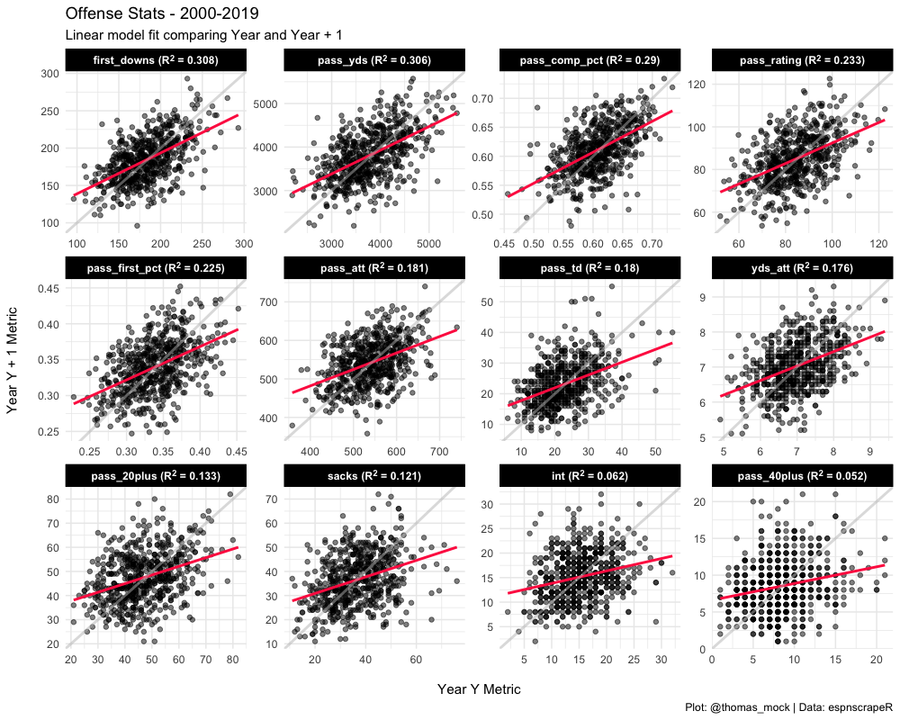
─ Session info ───────────────────────────────────────────────────────────────
 setting  value
 version  R version 4.2.0 (2022-04-22)
 os       macOS Monterey 12.2.1
 system   aarch64, darwin20
 ui       X11
 language (EN)
 collate  en_US.UTF-8
 ctype    en_US.UTF-8
 tz       America/Chicago
 date     2022-04-28
 pandoc   2.18 @ /Applications/RStudio.app/Contents/MacOS/quarto/bin/tools/ (via rmarkdown)
 quarto   0.9.294 @ /usr/local/bin/quarto

─ Packages ───────────────────────────────────────────────────────────────────
 package     * version date (UTC) lib source
 broom       * 0.8.0   2022-04-13 [1] CRAN (R 4.2.0)
 dplyr       * 1.0.8   2022-02-08 [1] CRAN (R 4.2.0)
 espnscrapeR * 0.6.5   2022-04-26 [1] Github (jthomasmock/espnscrapeR@084ce80)
 forcats     * 0.5.1   2021-01-27 [1] CRAN (R 4.2.0)
 ggplot2     * 3.3.5   2021-06-25 [1] CRAN (R 4.2.0)
 ggtext      * 0.1.1   2020-12-17 [1] CRAN (R 4.2.0)
 glue        * 1.6.2   2022-02-24 [1] CRAN (R 4.2.0)
 purrr       * 0.3.4   2020-04-17 [1] CRAN (R 4.2.0)
 readr       * 2.1.2   2022-01-30 [1] CRAN (R 4.2.0)
 sessioninfo * 1.2.2   2021-12-06 [1] CRAN (R 4.2.0)
 stringr     * 1.4.0   2019-02-10 [1] CRAN (R 4.2.0)
 tibble      * 3.1.6   2021-11-07 [1] CRAN (R 4.2.0)
 tidyr       * 1.2.0   2022-02-01 [1] CRAN (R 4.2.0)
 tidyverse   * 1.3.1   2021-04-15 [1] CRAN (R 4.2.0)

 [1] /Library/Frameworks/R.framework/Versions/4.2-arm64/Resources/library

──────────────────────────────────────────────────────────────────────────────